16.4 Line Integral Convolution (LIC) with Texture

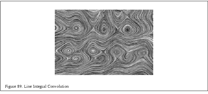
Line integral convolution is texture based technique for visualizing vector fields and has the advantage of being able to visualize large and detailed vector fields in a reasonable display area.

Line integral convolution involves selectively blurring a reference image as a function of the vector field to be displayed. The reference image can be anything, but to make the results clearer, is usually an spatially uncorrelated image (e.g., a noise image). The resulting image appears stretched and squished along the directions of the distorting vector field streamlines, visualizing the flow with a minimum of display resolution. Vortices, sources, sinks and other discontinuities are clear shown in the resulting image, and the viewer can get an immediate grasp of the flow fields ``big picture''.

In each case, you start with a vector field, sampled as a discrete grid of normalized vectors. You also need an image that is non-uniform and spatially uncorrelated, so correlations you apply to it will be more obvious. The goal is to process the image with the vector field, using line integral convolution, so you can visualize it. Note that in this technique, you will concentrate on the direction of the flow field, not its velocity; this is why the vector values at each gridpoint are normalized.

The processed image can be calculated directly using a special convolution technique. A representative set of vector values on the vector grid are chosen. Special convolution kernels are created shaped like the local stream line at that vector by tracing local field flow forwards and backwards some user-defined distance. The resulting curve is used as a convolution kernel to convolve the underlying image. This process is repeated over the entire image using a sampling of the vectors in the vector field.

Mathematically, for each location $p$ in the input vector field, a parametric curve $P(p, s)$ is generated which passes through the location and follows the vector field for some distance in either direction. To create an output pixel $F'(p)$, a weighted sum of the values of the input image $F$ along the curve is computed. The weighting function is $k(x)$. Thus the continuous form of the equation is:

$$F'(p) = \frac{\int^L_{-L}F(P(p,s))k(s)ds}{\int^L_{-L}k(s)ds}$$

To discretize the equation, use values $P_{0..l}$ along the curve $P(p, s)$:

$$F'(p) = \frac{\sum^l_{i=0}F(P_i)h_i}{\sum^l_{i=0}h_i}$$