3.7 Constructive Solid Geometry with the Stencil Buffer

Next: 4 Geometry and Transformations Up: 3 Modeling Previous: 3.6 Capping Clipped Solids Contents

3.7 Constructive Solid Geometry with the Stencil Buffer

Before continuing, the it may help for the reader to be familiar with the concepts of stencil buffer usage presented in Section 8.6.

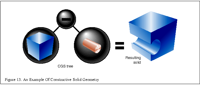
Constructive solid geometry (CSG) models are constructed through the intersection ( $\cap$ ), union ( $\cup$ ), and subtraction ( $-$ ) of solid objects, some of which may be CSG objects themselves[36]. The tree formed by the binary CSG operators and their operands is known as the CSG tree. Figure 13 shows an example of a CSG tree and the resulting model.

The representation used in CSG for solid objects varies, but we will consider a solid to be a collection of polygons forming a closed volume. ``Solid,'' ``primitive,'' and ``object'' are used here to mean the same thing.

$% latex2html id marker 1733 \fbox{\begin{tabular}{c} \vrule width 0pt height 0.1... ...Figure \thefigure . An Example Of Constructive Solid Geometry}\\ \end{tabular}}$

CSG objects have traditionally been rendered through the use of ray-casting, which is slow, or through the construction of a boundary representation (B-rep).

B-reps vary in construction, but are generally defined as a set of polygons that form the surface of the result of the CSG tree. One method of generating a B-rep is to take the polygons forming the surface of each primitive and trim away the polygons (or portions thereof) that do not satisfy the CSG operations. B-rep models are typically generated once and then manipulated as a static model because they are slow to generate.

Drawing a CSG model using stencil usually means drawing more polygons than a B-rep would contain for the same model. Enabling stencil also may reduce performance. Nonetheless, some portions of a CSG tree may be interactively manipulated using stencil if the remainder of the tree is cached as a B-rep.

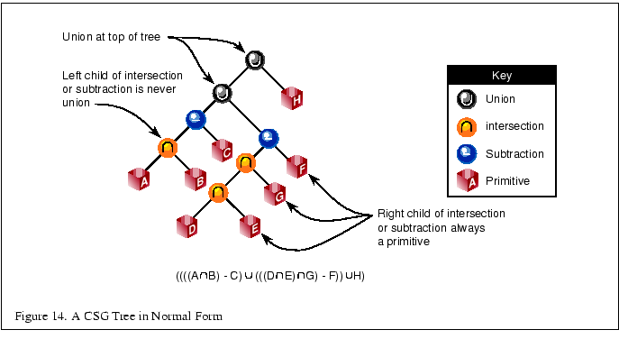
The algorithm presented here is from a paper by Tim F. Wiegand describing a GL-independent method for using stencil in a CSG modeling system for fast interactive updates. The technique can also process concave solids, the complexity of which is limited by the number of stencil planes available. A reprint of Wiegand's paper is included in the Appendix.

The algorithm presented here assumes that the CSG tree is in ``normal'' form. A tree is in normal form when all intersection and subtraction operators have a left subtree that contains no union operators and a right subtree that is simply a primitive (a set of polygons representing a single solid object). All union operators are pushed towards the root, and all intersection and subtraction operators are pushed towards the leaves. For example, $(((A \cap B) - C) \cup (((D \cap E) \cap G) - F)) \cup H$ is in normal form; Figure 14 illustrates the structure of that tree and the characteristics of a tree in normal form.

$% latex2html id marker 1749 \fbox{\begin{tabular}{c} \vrule width 0pt height 0.1... ...{5.7in}}{\small Figure \thefigure . A CSG Tree in Normal Form}\\ \end{tabular}}$

A CSG tree can be converted to normal form by repeatedly applying the following set of production rules to the tree and then its subtrees:

$X-(Y \cup Z) \; \rightarrow \; (X-Y)-Z$
$X \cap (Y \cup Z) \; \rightarrow \; (X \cap Y) \cup (X \cap Z)$
$X-(Y \cap Z) \; \rightarrow \; (X-Y) \cup (X-Z)$
$X \cap (Y \cap Z) \; \rightarrow \; (X \cap Y) \cap Z$
$X-(Y-Z) \; \rightarrow \; (X-Y) \cup (X \cap Z)$
$X \cap (Y-Z) \; \rightarrow \; (X \cap Y)-Z$
$(X-Y) \cap Z \; \rightarrow \; (X \cap Z)-Y$
$(X \cup Y)-Z \; \rightarrow \; (X-Z) \cup (Y-Z)$
$(X \cup Y) \cap Z \; \rightarrow \; (X \cap Z) \cup (Y \cap Z)$

X, Y, and Z here match either primitives or subtrees. Here is the algorithm used to apply the production rules to the CSG tree:

normalize(tree *t)
{
    if (isPrimitive(t))
        return;

    do {
        while (matchesRule(t))  /* Using rules given above */
            applyFirstMatchingRule(t);
        normalize(t->left);
    } while (!(isUnionOperation(t) ||
         (isPrimitive(t->right) &&
          ! isUnionOperation(T->left))));
    normalize(t->right);
}

Normalization may increase the size of the tree and add primitives that do not contribute to the final image. The bounding volume of each CSG subtree can be used to prune the tree as it is normalized. Bounding volumes for the tree may be calculated using the following algorithm:

findBounds(tree *t)
{
    if (isPrimitive(t))
        return;

    findBounds(t->left);
    findBounds(t->right);

    switch (t->operation){
      case UNION:
        t->bounds = unionOfBounds(t->left->bounds,
                                  t->right->bounds);
      case INTERSECTION:
        t->bounds = intersectionOfBounds(t->left->bounds,
                                         t->right->bounds);
      case SUBTRACTION:
        t->bounds = t->left->bounds;
    }
}

CSG subtrees rooted by the intersection or subtraction operators may be pruned at each step in the normalization process using the following two rules:

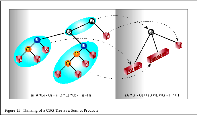
1.: If T is an intersection and not intersects(T->left->bounds, T->right->bounds), delete T.
2.: If T is a subtraction and not intersects(T->left->bounds, T->right->bounds), replace T with T->left.

The normalized CSG tree is a binary tree, but it is important to think of the tree rather as a ``sum of products'' to understand the stencil CSG procedure.

Consider all the unions as sums. Next, consider all the intersections and subtractions as products. (Subtraction is equivalent to intersection with the complement of the term to the right. For example, $A-B = A \cap \bar{B}$ .) Imagine all the unions flattened out into a single union with multiple children; that union is the ``sum.'' The resulting subtrees of that union are all composed of subtractions and intersections, the right branch of those operations is always a single primitive, and the left branch is another operation or a single primitive. You should read each child subtree of the imaginary multiple union as a single expression containing all the intersection and subtraction operations concatenated from the bottom up. These expressions are the ``products.'' For example, you should think of $((A \cap B)-C) \cup (((G \cap D) - E) \cap F) \cup H$ as meaning $(A \cap B-C) \cup (G \cap D - E \cap F) \cup H$ . Figure 15 illustrates this process.

$% latex2html id marker 1813 \fbox{\begin{tabular}{c} \vrule width 0pt height 0.1... ...gure \thefigure . Thinking of a CSG Tree as a Sum of Products}\\ \end{tabular}}$

At this time, redundant terms can be removed from each product. Where a term subtracts itself ( $A-A$ ), the entire product can be deleted. Where a term intersects itself ( $A \cap A$ ), that intersection operation can be replaced with the term itself.

All unions can be rendered simply by finding the visible surfaces of the left and right subtrees and letting the depth test determine the visible surface. All products can be rendered by drawing the visible surfaces of each primitive in the product and trimming those surfaces with the volumes of the other primitives in the product. For example, to render $A - B$ , the visible surfaces of A are trimmed by the complement of the volume of B, and the visible surfaces of B are trimmed by the volume of A.

The visible surfaces of a product are the front facing surfaces of the operands of intersections and the back facing surfaces of the right operands of subtraction. For example, in $(A - B \cap C)$ , the visible surfaces are the front facing surfaces of A and C, and the back facing surfaces of B.

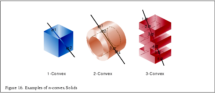
Concave solids are processed as sets of front or back facing surfaces. The ``convexity'' of a solid is defined as the maximum number of pairs of front and back surfaces that can be drawn from the viewing direction. Figure 16 shows some examples of the convexity of objects. The nth front surface of a k-convex primitive is denoted $A_{nf}$ , and the nth back surface is $A_{nb}$ . Because a solid may vary in convexity when viewed from different directions, accurately representing the convexity of a primitive may be difficult and may also involve reevaluating the CSG tree at each new view. Instead, the algorithm must be given the maximum possible convexity of a primitive, and draws the nth visible surface by using a counter in the stencil planes.

$% latex2html id marker 1839 \fbox{\begin{tabular}{c} \vrule width 0pt height 0.1... ...{\small Figure \thefigure . Examples of {\it n}-convex Solids}\\ \end{tabular}}$

The CSG tree must be further reduced to a ``sum of partial products'' by converting each product to a union of products, each consisting of the product of the visible surfaces of the target primitive with the remaining terms in the product.

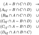
For example, if A, B, and D are 1-convex and C is 2-convex:

$\begin{eqnarray*} (A - B \cap C \cap D) & \rightarrow &\\ (A_{0f} - B \cap C \c... ...ap A - B \cap D) & \cup & \\ (D_{0f} \cap A \cap B \cap C ) & & \end{eqnarray*}$

Because the target term in each product has been reduced to a single front or back facing surface, the bounding volumes of that term will be a subset of the bounding volume of the original complete primitive. Once the tree is converted to partial products, the pruning process may be applied again with these subset volumes.

In each resulting child subtree representing a partial product, the leftmost term is called the ``target'' surface, and the remaining terms on the right branches are called ``trimming'' primitives.

The resulting sum of partial products reduces the rendering problem to rendering each partial product correctly before drawing the union of the results. Each partial product is rendered by drawing the target surface of the partial product and then ``classifying'' the pixels generated by that surface with the depth values generated by each of the trimming primitives in the partial product. If pixels drawn by the trimming primitives pass the depth test an even number of times, that pixel in the target primitive is ``out,'' and discarded. If the count is odd, the target primitive pixel is ``in,'' and kept.

Because the algorithm saves depth buffer contents between each object, we optimize for depth saves and restores by drawing as many of target and trimming primitives for each pass as we can fit in the stencil buffer.

The algorithm uses one stencil bit ( $S_p$ ) as a toggle for trimming primitive depth test passes (parity), n stencil bits for counting to the nth surface ( $S_{count}$ ), where n is the smallest number for which $2^n$ is larger than the maximum convexity of a current object, and as many bits are available ( $S_a$ ) to accumulate whether target pixels have to be discarded. Because $S_{count}$ will require the GL_ INCR operation, it must be stored contiguously in the least-significant bits of the stencil buffer. $S_p$ and $S_{count}$ are used in two separate steps, and so may share stencil bits.

For example, drawing two 5-convex primitives requires one $S_p$ bit, three $S_{count}$ bits, and two $S_a$ bits. Because $S_p$ and $S_{count}$ are independent, the total number of stencil bits required is 5.

Once the tree is converted to a sum of partial products, the individual products are rendered. Products are grouped together so that as many partial products can be rendered between depth buffer saves and restores as the stencil buffer has capacity.

For each group, writes to the color buffer are disabled, the contents of the depth buffer are saved, and the depth buffer is cleared. Then, every target in the group is classified against its trimming primitives. The depth buffer is then restored, and every target in the group is rendered against the trimming mask. The depth buffer save/restore can be optimized by saving and restoring only the region containing the screen-projected bounding volumes of the target surfaces.

for each group
    glReadPixels(...);
    <classify the group>
    glStencilMask(0);   /* so DrawPixels won't affect Stencil */
    glDrawPixels(...);
    <render the group>

Classification consists of drawing each target primitive's depth value and then clearing those depth values where the target primitive is determined to be outside the trimming primitives.

glClearDepth(far);
glClear(GL_DEPTH_BUFFER_BIT);
a = 0;
for (each target surface in the group)
    for (each partial product targeting that surface)
        <render the depth values for the surface>
        for (each trimming primitive in that partial product)
            <trim the depth values against that primitive>
        <set Sa to 1 where Sa = 0 and Z < Zfar>
        a++;

The depth values for the surface are rendered by drawing the primitive containing the the target surface with color and stencil writes disabled. ( $S_{count}$ ) is used to mask out all but the target surface. In practice, most CSG primitives are convex, so the algorithm is optimized for that case.

if (the target surface is front facing)
    glCullFace(GL_BACK);
else
    glCullFace(GL_FRONT);

if (the surface is 1-convex)
    glDepthMask(1);
    glColorMask(0, 0, 0, 0);
    glStencilMask(0);
    <draw the primitive containing the target surface>
else
    glDepthMask(1);
    glColorMask(0, 0, 0, 0);
    glStencilMask(Scount);
    glStencilFunc(GL_EQUAL, index of surface, Scount);
    glStencilOp(GL_KEEP, GL_KEEP, GL_INCR);	
    <draw the primitive containing the target surface>
    glClearStencil(0);
    glClear(GL_STENCIL_BUFFER_BIT);

Then each trimming primitive for that target surface is drawn in turn. Depth testing is enabled and writes to the depth buffer are disabled. Stencil operations are masked to $S_p$ and the $S_p$ bit in the stencil is cleared to 0. The stencil function and operation are set so that $S_p$ is toggled every time the depth test for a fragment from the trimming primitive succeeds. After drawing the trimming primitive, if this bit is 0 for uncomplemented primitives (or 1 for complemented primitives), the target pixel is ``out,'' and must be marked ``discard,'' by enabling writes to the depth buffer and storing the far depth value ( $Z_f$ ) into the depth buffer everywhere that the $S_p$ indicates ``discard.''

glDepthMask(0);
glColorMask(0, 0, 0, 0);
glStencilMask(mask for Sp);
glClearStencil(0);
glClear(GL_STENCIL_BUFFER_BIT);
glStencilFunc(GL_ALWAYS, 0, 0);
glStencilOp(GL_KEEP, GL_KEEP, GL_INVERT);
<draw the trimming primitive>
glDepthMask(1);

Once all the trimming primitives are rendered, the values in the depth buffer are $Z_f$ for all target pixels classified as ``out.'' The $S_a$ bit for that primitive is set to 1 everywhere that the depth value for a pixel is not equal to $Z_f$ , and 0 otherwise.

Each target primitive in the group is finally rendered into the framebuffer with depth testing and depth writes enabled, the color buffer enabled, and the stencil function and operation set to write depth and color only where the depth test succeeds and $S_a$ is 1. Only the pixels inside the volumes of all the trimming primitives are drawn.

glDepthMask(1);
glColorMask(1, 1, 1, 1);
a = 0;
for (each target primitive in the group)
    glStencilMask(0);
    glStencilFunc(GL_EQUAL, 1, Sa);
    glCullFace(GL_BACK);
    <draw the target primitive>
    glStencilMask(Sa);
    glClearStencil(0);
    glClear(GL_STENCIL_BUFFER_BIT);
    a++;

Further techniques are available for adding clipping planes (half-spaces), including more normalization rules and pruning opportunities [105]. This is especially important in the case of the near clipping plane in the viewing frustum.

Source code for dynamically loadable Inventor objects implementing this technique is available at the Martin Center at Cambridge web site [106].

Next: 4 Geometry and Transformations Up: 3 Modeling Previous: 3.6 Capping Clipped Solids Contents

2001-01-10